Single SNS junction¶

We want to calculate for an SNS junction:

The density of states for a given phase difference
The supercurrent-phase relation at a low temperature

Loading libraries¶

First, libraries need to be loaded:

from scipy import *
import usadel1 as u

Specifying the geometry¶

All calculations start with a geometry specification. An SNS junction can be modeled with two S-terminals and one N-wire:

geometry = u.Geometry(nwire=1, nnode=2)

geometry.t_type = [u.NODE_CLEAN_S_TERMINAL, u.NODE_CLEAN_S_TERMINAL]
geometry.w_type = [u.WIRE_TYPE_N]

The wire is connected to both terminals:

geometry.w_ends[0,:] = [0, 1]

Note that all indices are zero-based; the first terminal is 0 and the second 1.

Moreover, currently only clean interface boundary conditions are implemented. In principle, these would be straightforward to add; the place to put them would be in sp_equations.f90.

Then, assign a phase difference and energy gap for the terminals:

geometry.t_delta = [100, 100]
geometry.t_phase = [-.25*pi, .25*pi]

and set wire properties

geometry.w_length = 1
geometry.w_conductance = 1

Solving DOS¶

Next, the spectral equations can be solved, and results saved to a file:

solver = u.CurrentSolver(geometry)

solver.set_tolerance(sp_tol=1e-8)
solver.solve_spectral()
solver.save('sns-spectral.h5')

To capture the SNS junction minigap edge correctly at phase differences $\varphi>0.7\pi$ , we need to set a stricter tolerance $10^{-8}$ than the default $10^{-4}$ for the spectral solver. This has an impact on speed, however.

The results can be inspected with any program that can read HDF5 files, for example Matlab (use the supplied scripts/h5load.m script to load HDF5 files), or Python:

a, b = solver.spectral.a, solver.spectral.b
E, x = solver.spectral.E, solver.spectral.x
dos = real((1 + a*b)/(1 - a*b))

The solver object has attributes spectral, coefficient, kinetic that contain the solutions (Riccati parameters) $a$ , $b$ to the spectral equations, the kinetic coefficients, $D_L$ , $D_T$ , ${\cal T}$ , $j_S$ , and the solutions to the kinetic equations, $f_L$ , , $f_T$ . The Green function is parameterized in a mixed Riccati–distribution function scheme

$\hat{G}^R = \frac{1}{1 - a b} \begin{pmatrix} 1 + a b & 2 a \\ -2 b & -(1 + a b) \end{pmatrix}$

$\hat{G}^K = (\hat{G}^R - \hat{G}^A) f_L + (\hat{G}^R\hat{\tau}_3 -\hat{\tau}_3 \hat{G}^A) f_T$

Plot the DOS in the N-wire (lines for different positions are offset from each other):

import matplotlib.pyplot as plt
j = arange(0, 101, 2)
plt.plot(E[:,None] - 0.5*j[None,:], dos[:,0,::2] + 0.08*j[None,:], 'k-')
plt.xlabel('$E/E_T$'); plt.ylabel('$n/n_N$')
plt.ylim(0, 15); plt.xlim(-50, 300)
plt.savefig('dos.eps')

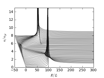
There is the minigap, already reduced by the finite phase difference.

Current-phase relation¶

First, we want to switch to a faster solver:

solver.set_solvers(sp_solver=u.SP_SOLVER_TWPBVP)

The default one is u.SP_SOLVER_COLNEW; there are some cases where TWPBVP does not converge, so it is not the default.

Current-phase relation can be calculated as follows:

phi = linspace(0, pi, 50)
I_S = zeros([50])

geometry.t_t = 1e-6 # Zero temperature

for j, p in enumerate(phi):
    geometry.t_phase = array([-.5, .5]) * p
    solver.solve()
    Ic, Ie = solver.get_currents(ix=0)
    I_S[j] = Ic[0]

savetxt('sns-I_S.dat', c_[phi, I_S])

What we do here is:

loop over different values of phases
change the phase difference in the geometry object
solve the spectral equations for each phase difference
compute the currents in the wire, at grid position 0
save the result to a file as two columns

The result is:

plt.clf()
plt.plot(phi/pi, I_S, 'k-')
plt.xlabel(r'$\varphi/\pi$'); plt.ylabel('$e R_N I_S / E_T$')

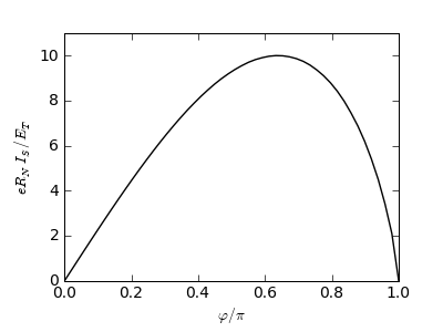
As we had $\Delta < \infty$ , the maximum $eR_NI_S$ does not reach $10.82 E_T$ .

Table Of Contents

Previous topic

Next topic

Navigation