Nonlocal thermovoltage

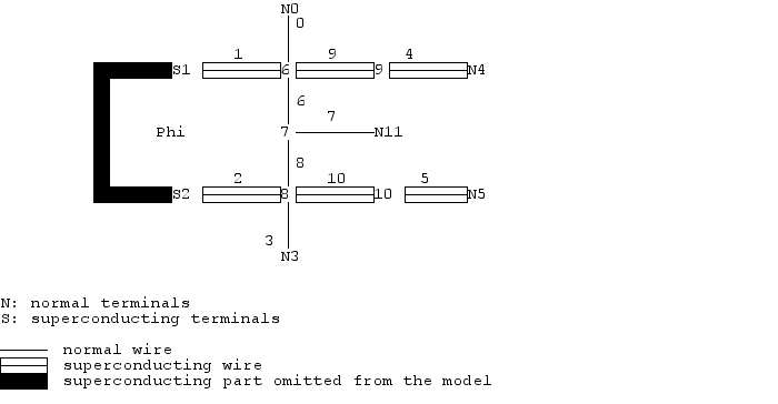
This roughly addresses the experiment in [CZ]. The structure studied could be roughly mapped on:

To try to model the actual experimental structure, resistive interface boundary conditions would be needed. In the calculations below, all interfaces are clean.

What’s calculated below is the potential at N4 when N11 is heated and all terminals float. All parameters have been chosen relatively arbitrarily and have not been specially tuned. You may wish to adjust them to see what happens.

An important question in the calculation is whether the change in the order parameter (caused by the applied heating) should be taken into account. One can argue that it does not contribute in the linear response:

1. The current entering terminal 4 is a function of the temperatures and potentials of the N-terminals, and a functional of the order parameter:

   

   Here, is a function of and . It is understood that the dependence from and arguments in is that obtained from a calculation with a fixed (possibly non-self-consistent) .

2. In the linear response the above is written as

   

   where the (functional) derivatives are evaluated at equilibrium, holding all other variables constant.

3. Because at equilibrium for any , , and the first term above vanishes.

Similarly for currents , , , . Hence, the thermovoltage does not contain any contribution from the linear-response change of the order parameter, and can be calculated directly from the Usadel equation without a need for nonequilibrium self-consistency.

This means that the only effect of using a self-consistent order parameter is that it tunes the diffusion and decay constants and the spectral supercurrent. I’d expect this effect to not cause any qualitative changes.

See also

example-nonlocal-thermovoltage.py

[CZ]	P. Cadden-Zimansky, J. Wei, V. Chandrasekhar, Nature Phys. 5, 393 (2009).

Geometry specification & code

See the example-nonlocal-thermovoltage.py in the scripts subdirectory; calculation goes as in Thermoelectricity in 4-probe structure.

The only addition is the optional self-consistent iteration for the order parameter (not taking into account the linear-response part ):

for T in logspace(log10(dT + 1e-4), log10(10), n_T):
    # Optional self-consistent iteration
    if do_selfconsistent_iteration:
        g.t_mu = 0
        g.t_t = T
        it = u.self_consistent_matsubara_iteration(g)
        #it = u.self_consistent_realtime_iteration(solver)
        for k, d, I_error in it:
            print "%% Self-consistent iteration %d (residual %g)" % (
                k, d.residual_norm())
            if (d.relative_residual_norm() < 1e-4 and I_error < 1e-5):
               break
        else:
            raise RuntimeError("Self-cons. iteration didn't converge!")

        solver.solve_spectral()
        solver.calculate_G()
        solver.save("nonlocal_thermovoltage_T_%.2f.h5" % T)

Here, we create an iterator corresponding to the Matsubara iteration, and iterate until stops changing.

Results

The calculation yields a finite thermovoltage at terminal 4 in response to heating in terminal 11.

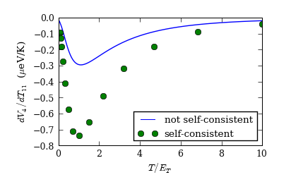
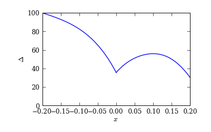
The result with a self-consistent (equilibrium) order parameter shows a larger thermovoltage, but this is only because the order parameter is significantly suppressed from the bulk value in the superconducting wires 1—9 (assumed of dimensionless length 0.2):

What occurs can be understood in a simple way: a finite potential () is induced at node 6 via the usual mechanism, and it propagates (as a non-equilibrium sub-gap excitation) through the superconducting wire, causing a potential to be induced to floating terminal 4. This is the clean-interface analogue of the crossed Andreev reflection. Propagation of the excitation is easily seen by looking at in wire 9:

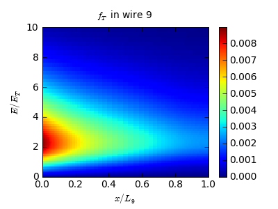
How large the effect is depends on how long the superconducting piece between 6–9 is, and the magnitude should decay exponentially as the length increases, due to charge mode relaxation. The characteristic length scale is not the inelastic relaxation length, because everything happens below the gap. Instead, it is proportional to the superconducting coherence length, as can be seen from the form of the sink terms in the Usadel equation:

The latter term participates in converting the sub-gap excitation to supercurrent, and the coefficient is large below the gap even deep in the superconductor where the phase of the order parameter . It is clear that the length scale corresponding to decay of must be proportional to .